Skip to main content
CHE155
Syllabus
Installation
Weeks:
1
2
3
4
5
6
7
8
9
10
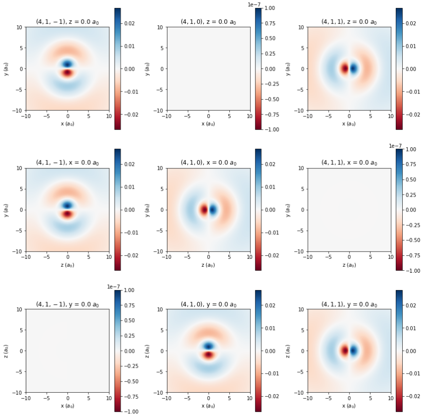
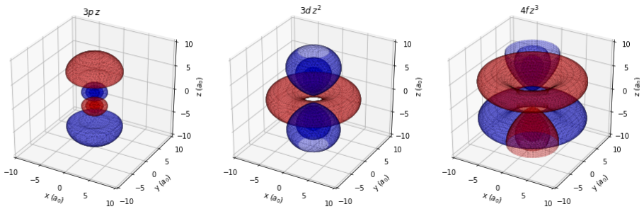
Week 2: Visualizing Hydrogen Atomic Orbitals
Overview
Background
Further Reading
Notebooks