Week 7: Molecular Structure and Chemical File Formats
Overview and Objectives
In the second half of the course, we will learn how to use two very important classes of theoretical / computational chemistry tools: quantum chemistry and molecular dynamics. These tools are used by research groups around the world to investigate all different kinds of chemical and physical processes, including studying the mechanisms of organic and inorganic reactions, simulating spectra across all regions of the electromagnetic spectrum, predicting the binding constants of proteins and small molecules, as well as predicting and optimizing material properties, and much more.
Although programming experience is not required to run basic calculations, there is a great amount of overlap between computational tools and programming, and anyone that does computational chemistry research would greatly benefit from understanding programming concepts and having some programming skills. For one, programming skills are important to most projects that involve developing theoretical methods, because in order for many new theories to be useful they need to be implemented in a computationally efficient way. Secondly, programming is powerful because it enables automation of repetitive tasks, which is needed for any computational research project that involves running large numbers of calculations and analyzing the results.
Because the development of new theoretical methods requires a level of understanding of quantum mechanics beyond the scope of this course, we will mainly focus on how to use existing computational chemistry tools in connection with Python programming. You will learn how to use quantum chemistry and molecular dynamics tools, both “manually” (i.e. making input files with a text editor and running programs on the command line) and “programmatically” (i.e. using Python programming to automate the running of calculations and analysis). The programs we’ll be using can be used directly from the command line as well as from inside a Jupyter notebook, providing two convenient points of entry for different types of projects.
The main learning objective of this week is to understand the basic elements of molecular structures and working with chemical file formats. All computational chemistry software tools work with files, therefore it is important to be able to store molecular structures and associated information in files. You will learn about the various file formats that molecular structures can be represented in, including the information that is contained (or not contained) in each different type of file. You will also learn how to visualize molecular structures in 3-D, how to access molecular structures on the Internet from public databases as well as subscription databases made available through the UC Davis library, and how to build molecular structures of your own. This in turn will form the foundation of running quantum chemistry calculations and molecular dynamics simulations that you will learn about starting next week.
Background

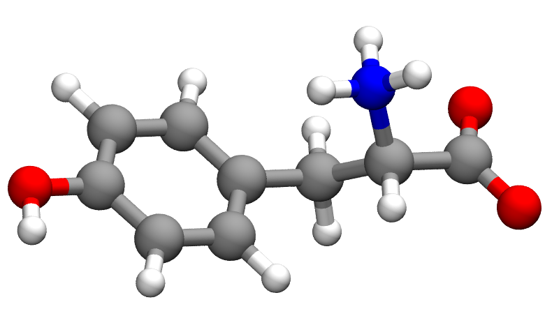
To start with, it’s important to make the distinction between 2D and 3D structures. A 2D and 3D structure of the same molecule (tyrosine in biologically occurring form) are shown above. These pictures are actually visualizations of the chemical data that is stored in the file. The source data looks like the following for the 2D and 3D structures:
2D (SMILES format):
[NH3+][C@@H](Cc1ccc(O)cc1)C([O-])=O
3D (xyz format):
24
Comment line
 O    -3.8866403600    -1.7797734900    -0.0278148700
 O    -4.3292469900     0.1251764400    -1.2123262200
 O     4.1256000000     0.6470000000     0.3613000000
 N    -1.9614224500     0.0607000600     1.2408205800
 C    -2.1878448800    -0.1499573500    -0.2239791300
 C    -1.1191000000    -1.1378000000    -0.7060000000
 C     0.2852000000    -0.6605000000    -0.4203000000
 C     0.7179000000     0.5375000000    -0.9650000000
 C     1.1132000000    -1.4292000000     0.3812000000
 C    -3.6093968200    -0.6499615500    -0.5219072200
 C     2.0143000000     0.9790000000    -0.7008000000
 C     2.4097000000    -0.9877000000     0.6455000000
 C     2.8603000000     0.2163000000     0.1044000000
 H    -2.0362863600     0.8331754200    -0.6852448600
 H    -1.2209623600    -1.3322340500    -1.7826794900
 H    -1.2645889900    -2.1143746600    -0.2238864400
 H    -2.6350215100     0.7362064400     1.6259500700
 H    -1.0193960400     0.4285713800     1.4296958300
 H    -2.0663528500    -0.8148760800     1.7708467600
 H     0.0753000000     1.1359000000    -1.6034000000
 H     0.7704000000    -2.3669000000     0.8089000000
 H     2.3542000000     1.9175000000    -1.1304000000
 H     3.0639000000    -1.5859000000     1.2739000000
 H     4.2676000000     1.4959000000    -0.0918000000
SMILES string - a representation of 2D structure
The text form of the 2D structure, called a SMILES string, contains information on how the atoms in the molecule are bonded to one another. The SMILES string also contains information about the stereochemistry of the chiral center (the alpha carbon), as well as some information about the Lewis structure of the system: the carboxylate group has a double bond and a formal minus charge, and the phenol side chain is aromatic. Hydrogen atoms are not always explicitly specified in the string, because many hydrogens are implicitly understood to exist in the structure according to normal valence assumptions.
The main convenience of the SMILES format is due to its small size, it can be easily transferred (i.e. cut, pasted, uploaded, downloaded, used in a search, etc.). It is usually not necessary to come up with a string “by hand”, even though in principle that is possible. More often, you can always import or export the chemical structure from a tool such as ChemDraw which has a free-to-use Web interface, or PubChem which is a chemical database maintained by the NIH. For those who are interested, the basic principles of how SMILES strings encode chemical structures is described in the Daylight SMILES theory documentation.
Quick exercise: Starting from any food or drink item that you have handy, look up one of the ingredients on Wikipedia or PubChem.
The ingredient you search for needs to be a small molecule (e.g. riboflavin or vanillin) and not something more general (e.g. flour, milk or spices).
(a) Write the name of the molecule as listed in the ingredients list on your answer sheet.
(b) Copy the SMILES string from the PubChem or Wikipedia entry for the molecule and paste it onto your answer sheet. Now go to the ChemDraw or PubChem structure drawing tool, find the tool for loading a SMILES string, and paste your string into the box. Make a substitution of your choice (e.g. change a methyl group to a trifluoromethyl group).
(c) Take a screenshot of the resulting structure, and include both your screenshot and a written description of your substitution on your answer sheet. Your description does not need to include formal atom numbering, and it will be sufficient to say, for example, “substituted trifluoromethyl for methyl group”.
(d) Export the SMILES string from the structure drawing tool and paste it into your answer sheet. You have now learned the basics of converting 2D chemical structures to and from SMILES strings, as well as where to find SMILES strings corresponding to known molecules on the Web.
.xyz file - basic 3D structure
The 3D structure on the other hand contains the Cartesian coordinates of each atom in 3-dimensional space. We can quickly see that the 3D structure has information not contained in the 2D structure, as there are now precise and quantitative numbers for the geometric details of the molecule, such as interatomic distances, angles, etc. Also, it is possible for many molecules of intermediate or larger size to possess multiple valid 3D structures or “conformations”, which are qualitatively different 3D structures that are consistent with the same 2D structure. Molecules that possess multiple conformations often owe their flexibility to rotatable bonds (these can be single or double bonds), and it is common to work with multiple 3D structures of the same molecule when comparing different conformations or working with a simulation trajectory (a trajectory is an evolving sequence or movie of 3D structures produced by a computer simulation.)
The .xyz format is one of the simplest ways to store 3D information.
The first line in the file is an integer that states the number of atoms in the structure, which assists programs with parsing the file, especially programs written in languages where memory allocation is important such as C or Fortran.
The second line is a comment and anything can be written here.
This is followed by a number of lines each containing a string for the atomic symbol followed by three floating point numbers for the Cartesian coordinates in Angstrom; it is important that the number of these “data lines” equals the number in the first line.
Multiple structures can be included in a single .xyz file by simply concatenating multiple files together.
Although the Cartesian coordinates and comment line can vary between structures in a single .xyz file, generally the number of atoms, the atomic symbols and ordering of atoms cannot change.
In contrast with 2D structures, the .xyz file contains no explicit information about chemical bonding, stereochemistry, or formal charges.
Although it is often possible to infer some information by examining the relative locations of atoms in space (e.g. a C and H atom separated by 1 Angstrom are probably bonded), this is not always possible, so the 3D structure by itself is considered to be “missing” some chemical information.
In quantum chemistry and density functional theory, the chemical bonding and all electronic properties of the system are obtained by running a calculation starting from the 3D structure and two additional numbers: the charge (an integer) and spin multiplicity (a positive integer).
(As a reminder, the spin multiplicity is equal to the number of unpaired electrons plus one, so a typical neutral, non-radical organic molecule has charge 0 and multiplicity 1).
Indeed, quantum chemistry is somewhat detached from the chemical information in 2D structures because neither is there any chemical information input into the calculation, nor is it straightforward to extract this information from the calculation results.
So if your research project involves running lots of quantum chemistry calculations, you may only need to need to draw the 2D structures when giving presentations and writing papers.
.pdb file format - 3D structure with some chemical information
Outside of quantum chemistry however, it is important to have the ability for 3D structures to include some chemical information. The .pdb file is a file format used by the Protein Databank (also called the PDB), the standard website for downloading protein structures determined from X-ray crystallography, NMR spectroscopy, cryo-EM microscopy, and other methods. In a .pdb file, each line describing atomic coordinates also contains some other information:
ATOM    757  N   TYR A 100      26.251  43.232  17.976  1.00  8.95           N
ATOM    758  CA  TYR A 100      25.808  42.007  18.632  1.00 13.56           C
ATOM    759  C   TYR A 100      24.860  42.303  19.794  1.00 15.66           C
ATOM    760  O   TYR A 100      23.813  41.679  20.023  1.00 12.33           O
ATOM    761  CB  TYR A 100      27.046  41.234  19.175  1.00 12.23           C
ATOM    762  CG  TYR A 100      27.860  40.460  18.135  1.00  7.98           C
ATOM    763  CD1 TYR A 100      27.256  39.716  17.122  1.00 10.03           C
ATOM    764  CD2 TYR A 100      29.252  40.417  18.191  1.00  9.54           C
ATOM    765  CE1 TYR A 100      28.005  38.972  16.201  1.00  7.43           C
ATOM    766  CE2 TYR A 100      30.012  39.686  17.277  1.00 13.65           C
ATOM    767  CZ  TYR A 100      29.392  38.953  16.268  1.00  9.23           C
ATOM    768  OH  TYR A 100      30.130  38.245  15.363  1.00 11.17           O
ATOM    769  N   GLU A 101      25.255  43.320  20.529  1.00 17.62           N
ATOM    770  CA  GLU A 101      24.468  43.720  21.670  1.00 18.23           C
ATOM    771  C   GLU A 101      23.106  44.168  21.313  1.00 15.89           C
After the ATOM, there are five fields of information: 757: the sequential atom number in the file, N: the atom name, TYR: the residue name - in the case of amino acids it’s the standard three-letter code, A: the chain identifier, and 100: the residue number.
In the file this snippet was taken from, there were 756 other atoms and 99 other residues before this one.
A central concept in .pdb files is the residue, which could mean either a small molecule or a subunit of a larger molecule, like an amino acid in a protein (the name derives from condensation reactions, as the “residue” is the part of the monomer that remains attached to the polymer.)
Each residue has a standardized list of atoms and a list of bonds between atoms, therefore the .pdb file carries some chemical information about the molecules it contains in addition to the 3D coordinates.
The most commonly occuring residues in .pdb files are the standard 20 amino acids, water molecules, and ions (e.g. Na+ / Cl-), but many other residues and small molecules can be included in the structure as well.
A .pdb file may contain carbohydrates, nucleic acids and lipids, small molecule hormones and drug-like compounds, and enzyme active sites that may contain transition metal ions or clusters.
A chain is comprised of multiple residues bonded together, and a single .pdb file may contain multiple chains if the protein structure is a dimer, trimer or other assembly.
Note that structures downloaded from the Protein Databank often do not contain hydrogen atoms, as they are difficult to resolve in X-ray crystallography experiments, and the hydrogens may have to be added back before one can run simulations.
NMR experiments on the other hand provide multiple structures complete with hydrogen atoms, mainly because of the different nature of the experiments and modeling software used to generate the structures.
Also, the .pdb file limits the precision of atomic coordinates to 0.001 Angstrom, which is more than sufficient for experiments, but is not enough for some theoretical applications.
In addition to being a file format for storing experimental structures, the .pdb format is often the starting point for molecular mechanics simulations. Many of the major molecular mechanics packages - AMBER, CHARMM, GROMACS, OpenMM, and others - make it relatively easy to use .pdb files as the entry point for setting up and running simulations. In addition, a number of software tools for molecular modeling makes it possible to view and edit the contents of .pdb files.
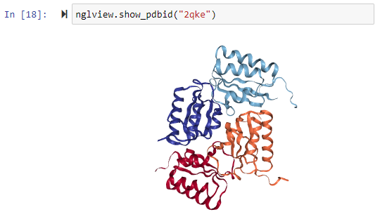
Because a PDB file can contain thousands of atoms, they are typically rendered using a cartoon representation that shows the protein secondary structure only (alpha-helix, beta-strand, or random coil.)
You can use the nglview package to view protein structures from the PDB by just entering the four-letter PDB ID, without having to download the file:
.cif file format - 3D structure with crystallographic information
Another example of a file format you may become familiar with in your research is the Crystallographic Information File (.cif).
This is another standard format for depositing experimental data, usually on small molecules from X-ray crystallography.
These files contain not only the 3D structure of the molecule(s) within the unit cell, but other information such as the lattice parameters of the crystallographic unit cell, the experimental methods used, uncertainty in the atomic positions, etc.
Generally, you would need to convert the .cif file into another format before it is possible to start doing any computer simulations.
Working with chemical file formats
There are lots of ways to work with these chemical file formats that certainly depends on the task or project at hand.
To start with, it’s good to know how to create files from scratch.
There exist a number of molecule editors that are capable of creating 2D and 3D chemical structures; one example is Avogadro, a free tool that allows one to build 3D structures and save to a number of file formats.
ChemDraw is a commonly used proprietary software package, mostly used to draw 2D structures for organic molecules (at least in my experience); it is also available for free with limited functionality on the Web.
Files such as .cif and .pdb deposited online are typically produced by specialized software that interprets crystallographic, NMR or other experimental data; we will not be talking about how these files are produced here.
It’s also important to know where to find existing chemical structures on the Web; many of these structures are determined experimentally. The Protein Databank (PDB) is a principal source of protein and biomolecular structures, and it provides a fully featured website for users to search for and download these structures in either .pdb or .cif format. For organic and inorganic molecules, two well-known and high-quality structure databases are the Cambridge Structural Database (CSD) based in the UK and the Inorganic Crystal Structure Database (ICSD) based in Germany. Both databases are searchable using the Access Structures web portal; however, the public searching tools are very limited, so you will need to connect to the website from campus or use the UC Davis VPN in order to access the paid advanced search tools.
A third important skill in working with chemical file formats is how to visualize the files.
Several of the web portals used for searching experimental structures have integrated viewers where you can view the 3D structure directly on the webpage.
Avogadro, mentioned above, is a useful viewer for small molecules.
VMD is a free software package that is used mostly for viewing bio-molecular simulation trajectories.
The nglview package is available to visualize 3D structures inside of Jupyter.
There are various other molecule viewers and editors available, and their features and licensing models vary substantially.
Examples of semi-free or commercial molecule viewers/editors that your instructor knows about include PyMol, MOE, GaussView, and Spartan; these software packages are often integrated with computational tools on the backend.
Last but not least, if you want to work with chemical file formats on a regular basis, you will need ways to process them on the command line or programmatically in side your Python code / Jupyter. You might want to convert a big batch of SMILES strings into .xyz files, for example. If you want to process chemical structures in more flexible ways, you may want to work with a library that not only can convert between file formats, but also represent the chemical structure as an object inside of your codes, much like a NumPy array or Matplotlib figure. Two freely available cheminformatic libraries that facilitate file format conversion and other processing of chemical structures are OpenBabel and RDKit. Note that the releases made available for download on SourceForge are often out of date by a few years. The conda package manager that we use to create the Python environment has the latest versions of RDKit and OpenBabel (the latest versions are 2021.03.1 and 3.1.1 at the time of this writing), and the latest source codes can be found on the corresponding GitHub repositories. Some examples of commercial cheminformatics toolkits used in industry include OpenEye and ChemAxon.
When working with these packages, make sure that you are using the correct version of the OpenBabel documentation/RDKit documentation, because an old version of the documentation will not have a complete list of the features (and may even describe obsolete features). Confusingly, the OpenBabel documentation homepage links to an older version of itself at the top of the page where it says “The latest version of this documentation is available in several formats from http://openbabel.org/docs/dev/ (the link points to documentation for an older version.)” When working with open source software, there will usually be more bugs and out-of-date webpages compared to commercial software because the developers are often maintaining the packages on their own free time.
Other file formats
There are many other file formats besides the ones described in this lesson. Nearly every quantum chemistry program (Gaussian, Q-Chem, Psi4, Turbomole, Orca, Molpro, GAMESS, TeraChem, etc.) has its own input and output file format. Molecular dynamics codes (AMBER, CHARMM, Gromacs, OpenMM, NAMD, LAMMPS, TINKER, etc.) may be a bit more standardized in their input formats (for example, many allow .pdb as a convenient entry point) but they also have many output formats; in particular there are several different trajectory file formats that are specialized for storing a large number of structures saved at intervals during the simulation. Examples of trajectory file formats include .xtc, .trr, .dcd, .netcdf and the list goes on. There are also file formats that combine 3D coordinate information with the chemical metadata found in 2D structures; .mol2 and .sdf are prominent examples of these.
Clearly, there is a wide variation in the file formats that are required by different applications, and that reflects the complexity of information that can be contained in a molecular structure. The simpler file formats tend to be more transferable and supported by a greater number of programs, but they might not contain sufficient information to support the needs of a project or a calculation. On the other hand, more complex file formats can hold more information about a molecule but also require more specialized software to read and write them. In any research project involving computation, it is important to become familiar with the file formats required by the simulation programs, and hopefully this tutorial has enabled you to become more agile with chemical file formats so that they can be of assistance in your research rather than a hindrance.