Week 4: Fitting Experimental Data to Models I

Overview and Objectives
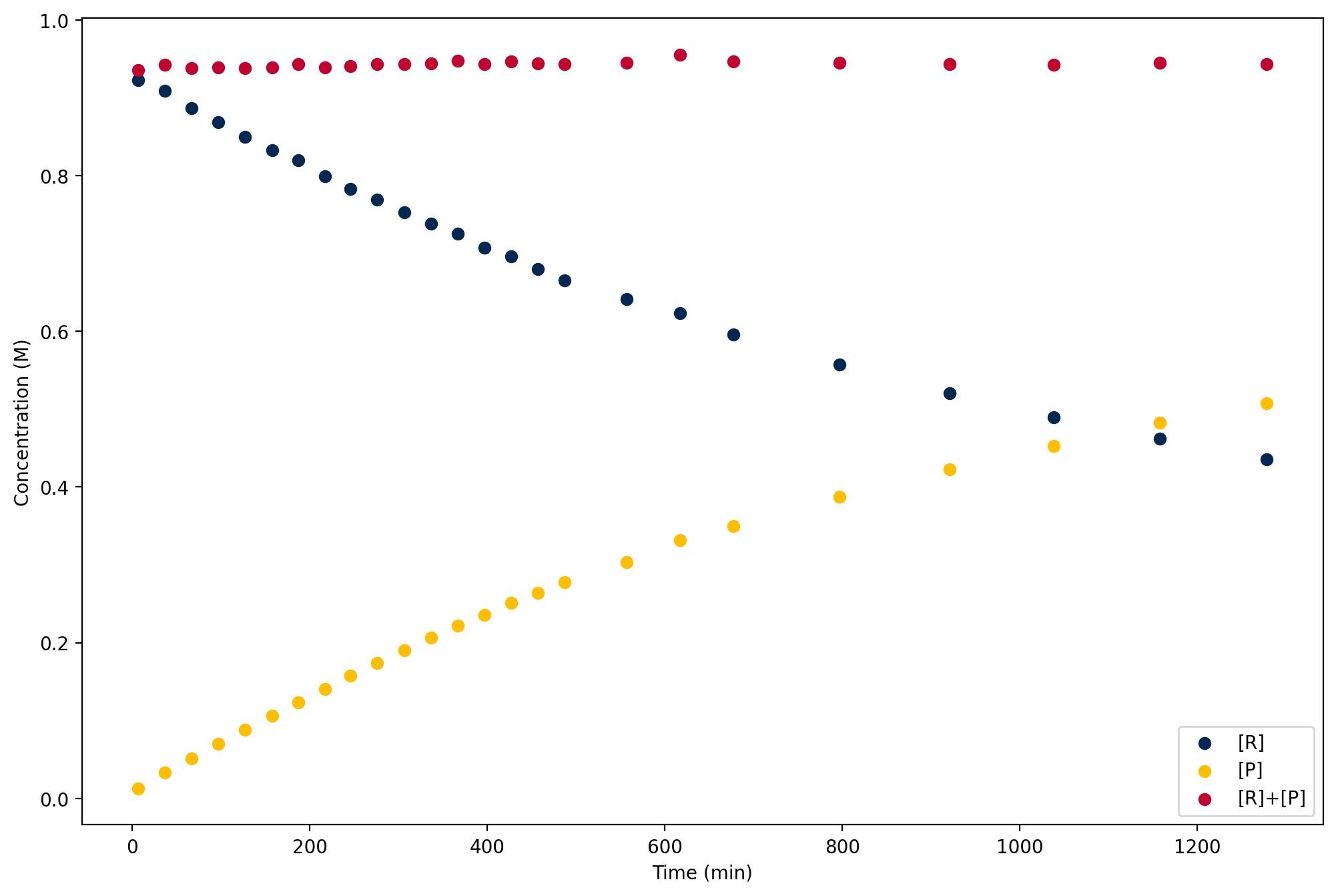
This week we will use Python to process real experimental data from Dr. Annaliese Franz’s research group at UC Davis. The data are from a series of Nuclear Magnetic Resonance (NMR) Spectroscopy measurements that aim to assess the kinetics of a chemical reaction in the presence of a catalyst (J. R. Jagannathan et al. (2019) Chem. Eur. J. 25, 14953-14958). Reactants and the catalyst are combined in a small tube and inserted into the spectrometer, then measurements are taken at a series of time points to monitor the concentrations of reactants and products. Analyzing the concentrations as a function of time provides insight into the behavior of the catalyst and the mechanism of the reaction.
In addition to data visualization with matplotlib, organization with pandas, and statistics with pingouin, we will also be exploring the use of two new scipy modules for analysis:
scipy.integratecontains a number of functions that can perform numerical integration. We will usetrapezoidandsimpson.scipy.optimizecontains algorithms for root finding, minimization, and maximization. We will usecurve_fitthis week, and will look at other functions in the future.
Background
POSS-catalyzed Indole Addition Kinetics

The data analysis for this week will be for the system shown above. Compound A (4-trifluoromethyl-trans-beta-nitrostyrene) is an electrophile that reacts with the nucleophile B (N-methylindole). C is the catalyst POSS-triol (phenyl polyhedral oligomeric silsesquioxane triol), and D is an internal standard that is used for concentration calibration during the spectroscopy, as we will discuss below. The reaction is monitored using \(^{19}\)F NMR spectroscopy, which can see molecules that contain F atoms. As a result, during the experiment, the concentrations of A, D, and the product E can be measured.
The goal of the experiment is to determine the rate of the reaction, and determine the reaction order with respect to compound A. The rate of a reaction is related to the concentration change per unit time for a molecule. For the reaction A + B \(\to\) E, the rate is:
\[ \text{Rate} = -\frac{\text{d}[\textbf{A}]}{\text{d}t} = -\frac{\text{d}[\textbf{B}]}{\text{d}t} = \frac{\text{d}[\textbf{E}]}{\text{d}t} = k[\textbf{A}]^x[\textbf{B}]^y \]
where [X] is the concentration of X, \(k\) is the rate coefficient, and \(x\) and \(y\) are the reaction orders for each reactant. The total reaction order is \(x+y\), and the orders for the reactants are often (though not always!) integers, and may be 0. If the reaction occurs in a single step, then the reactant orders are equal to their stoichiometric coefficients in the balanced chemical reaction, but this system involves a catalyst and likely several steps so the rate law needs to be determined experimentally. If the reaction is zero order in B, then the reaction rate may be able to fit a straight-line plot depending on the order in A (see the further reading for more details):
- Zero order: A graph of [A] vs time is linear with a slope of \(-k\)
- First order: A graph of ln [A] vs time is linear with a slope of \(-k\)
- Second order: A graph of 1/[A] vs time is linear with a slope of \(k\)
Nuclear Magnetic Resonance (NMR) Spectroscopy
NMR is a widely-used spectroscopic technique in chemistry. In NMR spectroscopy, a molecule of interest is placed into a strong magnetic field and irradiated by radiofrequency light. Nuclei that possess magnetic moments (e.g., \(^1\)H, \(^{13}\)C, \(^{19}\)F, and several others) experience Zeeman Splitting due to their orientation in the field. Here we are concerned with \(^{19}\)F, which is a spin-1/2 nucleus. Like an electron, a \(^{19}\)F nucleus can either be spin-up (+1/2) or spin-down (-1/2). In the magnetic field, the energies of the two spin states are different:
\[ \Delta E = \hbar\gamma B_0 \]
where \(\gamma\) is the gyromagnetic ratio of the \(^{19}\)F nucleus (251.662 x 10\(^6\) rad s\(^{-1}\) T\(^{-1}\)), \(\hbar\) is Planck’s constant divided by 2\(\pi\), and \(B_0\) is the strength of the magnetic field (in Tesla). The frequency of light that causes a transition can be calculated by setting the energy of a photon equal to the different in energy between the +1/2 and -1/2 nuclei. This gives the Larmor frequency, which is the frequency at which a peak will appear in the NMR spectrum for that nucleus.
\[ h\nu = \hbar\gamma B_0, \quad \nu = \frac{\gamma B_0}{2\pi} \]
When they are placed in a molecule, the fluorine nuclei are shielded from the external magnetic field by the electrons in the molecule. The amount of shielding depends on the details of the electronic environment, and consequently, F atoms at different locations within a molecule may have different Larmor frequencies, and F atoms in different molecules also have different Larmor frequencies. We can account for the shielding by introducing a shielding constant \(\sigma\) into the equation for the Larmor frequency:
\[ \nu = \frac{\gamma(1-\sigma)B_0}{2\pi} \]
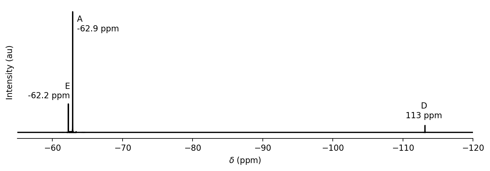
Shielding constants are typically small numbers (~10\(^{-4}\) - 10\(^{-6}\)). Instead of measuring Larmor frequencies and shielding constants directly, chemists typically measure the difference in frequency between a peak of interest and a reference molecule. this difference is referred to as a chemical shift (\(\delta\)) and is equivalent to the difference in shielding constants between the peak from the analyte molecule and the peak from the reference molecule. Because shielding constants are so small, the difference is multiplied by 10\(^6\) and reported in units of ppm. For fluorine NMR, the reference molecule is usually CFCl\(_3\). For the F-containing compounds in the indole addition reaction, the chemical shifts are approximately -62.9 ppm for A. -62.2 ppm for E, and -113 ppm for D. The three F atoms in the -CF\(_3\) groups have the same chemical shift.
The size of a peak in an NMR spectrum is proportional to the concentration of F nuclei at that chemical shift. More specifically the area \(A\) of the NMR peak for molecule X is proportional to (X) times the number of fluorine atoms with that chemical shift \(N_F\):
\[ A \propto [\textbf{X}]N_F \]
The area \(A\) can be measured from the NMR spectrum and then used to infer the relative concentration of a molecule. This can be done either by numerical integration or by curve fitting. An example \(^{19}\)F NMR spectrum from the indole addition reaction is shown below (by convention, NMR spectra are plotted with chemical shift increasing to the left).

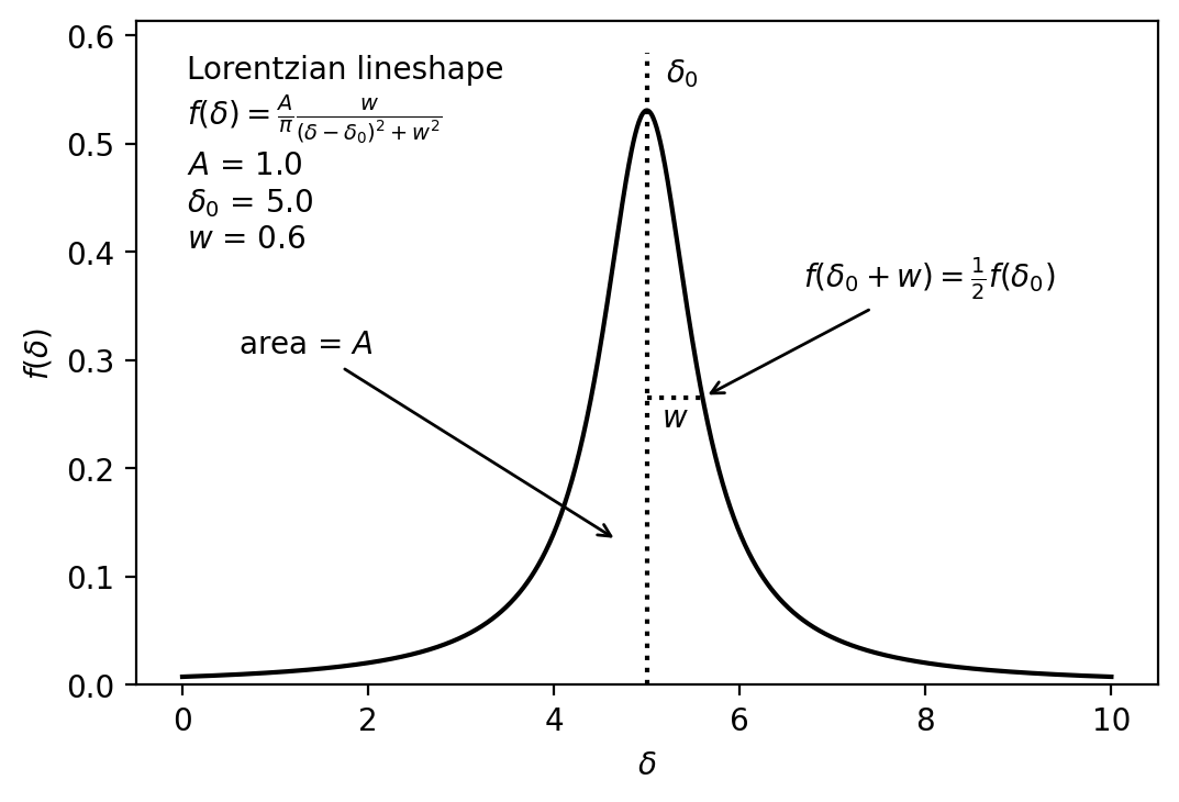
A single peak in an NMR spectrum has approximately a Lorentzian lineshape. In other words, the shape of the peak as a function of chemical shift is
\[ f(\delta) = \frac{A}{\pi}\frac{w}{(\delta - \delta_0)^2 + w^2} \]
- \(\delta\) is the chemical shift along the x axis of the NMR spectrum
- \(A\) is the total area of the peak
- \(w\) is the half width at half maximum (HWHM) of the peak, where \(f(\delta \pm w) = f(\delta_0)/2\).
- \(\delta_0\) is the exact center of the peak, where \(\delta = \delta_0\).

We can “fit” a lineshape function to the data by finding the values of \(A\), \(w\), and \(\delta_0\) that best match the shape of the experimental data using a nonlinear least squares routine.
Nonlinear Least Squares Fitting
Last week, we used linear regression to fit a line to experimental data. The key point was that the best fit line \(f(x)\) was the one that minimized the sum of the squares of the residuals; given data points \(x_i,y_i\), the goal is to minimize \(S\), the sum of the squares of the residuals \(r_i\):
\[ S = \sum_{i=1}^N r_i^2 = \sum_{i=1}^N (y_i - f(x_i))^2 \]
where the model function is evaluated at each \(x_i\) data point. In linear regression, the model function \(f(x_i)\) depends on a set of \(M\) parameters \(c_m\) that are multiplied by functions of the independent variable \(x\). An example is a polynomial function:
\[ f(x;c_0,c_1,\ldots,c_M) = c_0 x^0 + c_1 x^1 + \ldots + c_M x^M \]
However, when the parameters are more complicated than just multipliers of the dependent variable, the problem is nonlinear and more sophisticated algorithms must be employed. In the Lorentzian function above, the independent variable is \(\delta\) and the parameters are \(A\), \(w\), and \(\delta_0\). Because the equation cannot be written in a form in which each parameter is multiplied by a function of \(\delta\), fitting with this model function is a nonlinear least squares problem.
When the sum of squares of the residuals is minimized, the derivatives of \(S\) with respect to all of the parameters \(c_m\) are 0. Since there are \(M\) parameters, there are \(M\) equations that are 0 at the minimum:
\[ \frac{\partial S}{\partial c_m} = 2\sum_{i=1}^N r_i\frac{\partial r_i}{\partial c_m} = 0 \]
When the system is linear, these equations have a simple closed-form solution, but in a nonlinear problem the derivatives depend on the parameters and the independent variable, and there is no such solution that gives the values of the optimized parameters. However, given initial guesses for their values, the equations can be used to iteratively refine the values toward the values that minimize \(S\).
The system of equations is typically written using matrix-vector notation. Another way of saying that all of the derivatives are 0 is that the gradient vector is equal to 0. The gradient vector is just a vector whose elements are the derivatives with respect to each parameter. For the Lorentzian function, this would be:
\[ \frac{\partial S}{\partial \mathbf{c}} = \begin{bmatrix} \displaystyle \frac{\partial S}{\partial A} \\[1em] \displaystyle \frac{\partial S}{\partial w} \\[1em] \displaystyle \frac{\partial S}{\partial \delta_0} \end{bmatrix}, \quad \mathbf{c} = \begin{bmatrix} A \\[1em] w \\[1em] \delta_0 \end{bmatrix} \]
In the iterative procedure, at each step the parameter vector \(c\) is changed by an amount \(\Delta \mathbf{c}\). The sizes of the changes are estimated by a linear approximation that depends on the Jacobian Matrix \(\mathbf{J}\), which is an (\(M \times N\)) matrix whose elements are the derivative of each individual residual with respect to a parameter:
\[ \mathbf{J}_{ij} = \frac{\partial r_i}{\partial c_j} \]
Finally, the changes in parameter values \(\mathbf{\Delta c}\) for an iteration are the solutions to the equation
\[ (\mathbf{J}^T\mathbf{J})\mathbf{\Delta c} = \mathbf{J}^T \mathbf{\Delta r} \]
where \(\mathbf{J}^T\) is the transpose of the Jacobian matrix and \(\mathbf{\Delta r}\) is the vector of residuals. For the next iteration, the parameters are updated by adding \(\mathbf{c} + \mathbf{\Delta c}\), and then \(\mathbf{J}\) is recalculated, and the process repeated until the elements of the gradient vector become very small, or the parameter changes \(\mathbf{\Delta c}\) become small.
This week we will use scipy.optimize.curve_fit, which is an implementation of nonlinear least squares. We provide the function to be fitted to the data, the x and y data values to fit, and initial guesses for the parameters. The curve_fit function is able to estimate the Jacobian matrix via finite differences (or we can provide a function to calculate it), and returns the optimized parameter values and the covariance matrix, the latter of which gives an estimate of the parameter uncertainties. This will allow us to determine the peak areas in the NMR spectra in this week’s notebooks.
Further Reading
- J. R. Jagannathan et al. (2019) Chem. Eur. J. 25, 14953-14958
- Reaction Kinetics: A Summary - LibreTexts
- Introduction to NMR - LibreTexts
