Week 5: Fitting Experimental Data to Models II
Overview and Objectives
In this week’s notebook we are going to build our knowledge of fitting experimental data to model functions by exploring a more complicated problem in chemical kinetics. As you have learned in general chemistry, differential equations can be used to describe the rates of elementary chemical reactions in terms of a rate coefficient and the concentrations of reactants. When multiple reactions occur at the same time, the differential equations are coupled, and the integrated rate equations become more complicated.
We will analyze experimental data on the deuteration of H\(_3^+\) in an ion trap at 13.5 K from E. Hugo et al. (2009) J. Chem. Phys. 130, 164302. Initially we will use the scipy.optimize.curve_fit function, and then will move on to building a more complete model, which requires using the lower-level scipy.optimize.least_squares function.
Background
Deuteration of H\(_3^+\)
Molecular hydrogen is the most abundant molecule in the universe. In space, it can be ionized by cosmic rays to form H\(_2^+\), which in turn can react with H\(_2\) to make H\(_3^+\), the simplest polyatomic molecule. H\(_3^+\) is an extremely strong acid which can protonate nearly any neutral atom or molecule. These proton transfer reactions initiate a sequence of ion-molecule reactions which can form many of the ~200+ molecules which have been detected in space.
Deuterium, an isotope of hydrogen with an additional neutron, has a cosmic abundance of about \(10^{-5}\) relative to hydrogen. In other words, there is 1 D nucleus for every 100,000 H nuclei. However, in the coldest, darkest regions of space, astronomers have observed that the isotopic ratios of some molecules, e.g., [DCO\(^+\)]:[HCO\(^+\)], can be approximately 1! The origin of this deuterium enrichment can be traced back to H\(_3^+\), which reacts exothermically with HD. The table below shows a series of deuteration reactions, and the reaction energies are converted to Kelvin so that they can be compared with thermal energy \(k_b T\).
| Reaction | \(\Delta E / k_B\) (K) |
|---|---|
| H\(_3^+\) + HD \(\rightleftharpoons\) H\(_2\)D\(^+\) + H\(_2\) | \(-232\) |
| H\(_2\)D\(^+\) + HD \(\rightleftharpoons\) D\(_2\)H\(^+\) + H\(_2\) | \(-187\) |
| D\(_2\)H\(^+\) + HD \(\rightleftharpoons\) D\(_3^+\) + H\(_2\) | \(-234\) |
Based on these reaction energies, if the temperature is significantly below 187 K, the reverse reactions become slow enough to be ignored. In the regions of space where deuterium enrichment is observed, the temperature is ~10 K. Under these conditions, over time H\(_3^+\) is converted to D\(_3^+\), which can readily donate a D\(^+\) to other molecules. In order to model the chemistry occurring in space, it is important to know how fast these reactions occur at very low temperatures.
Ion Trap Experiments
An ion trap is a device that uses voltages to contain ions inside a fixed region. Because cations have a positive charge, they can be trapped by surrounding them with electrodes that are held at a positive voltage. In the experiment we will look at, the authors use a trap that consists of 22 rods arranged like a cylinder together with a pair of ring electrodes at either end of the cylinder. A simple schematic is shown below:

In this experiment, H\(_2\) gas is fed into an electrical discharge to produce ions (this is the ion source). A voltage is used to extract a beam of positively charged ions, which make their way into mass filter 1. The mass filter consists of 4 rods, a quadrupole, and they are driven with voltages that alternate at radiofrequencies. These voltages are tuned such that as the ions fly through, the quadrupole kicks out all ions with a mass:charge ratio different than 3. By the end of the first mass filter, only H\(_3^+\) remains (plus a tiny amount of HD\(^+\)).
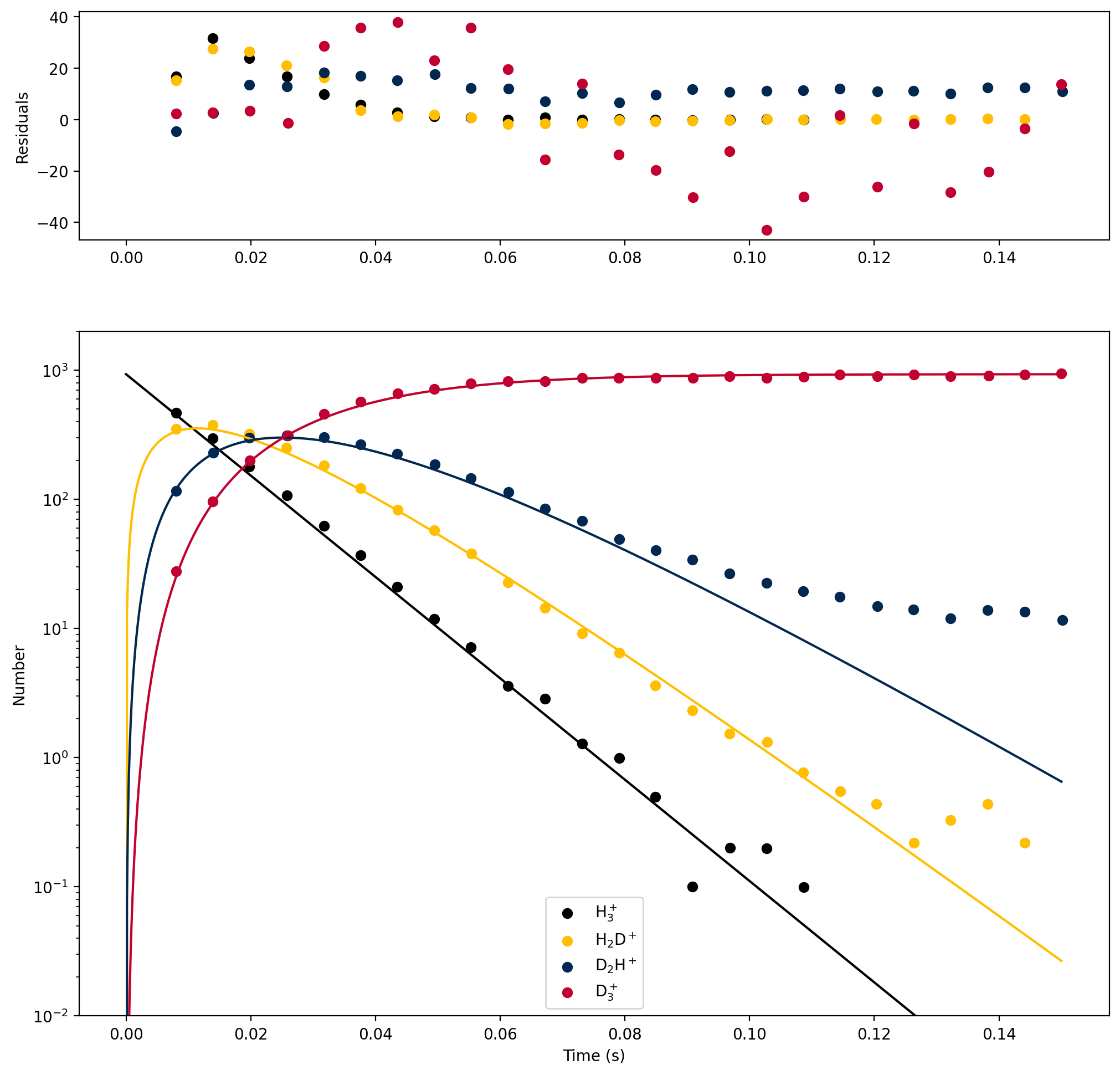
The H\(_3^+\) ions are admitted into the 22-pole trap by grounding the first ring electrode and raising the second to a positive voltage while applying radiofrequency voltages to the 22 rod electrodes to stop the ions from escaping. Once enough ions are inside the trap, the first ring electrode is put at a positive voltage to keep them inside and to stop any more ions from entering. Then the ions are gently cooled to 13.5 K by leaking in precooled He gas for a few milliseconds. Once the ions are cool, HD gas, also precooled, is let into the trap where it reacts with the H\(_3^+\) ions. After some time \(t\), the ions are pushed to the end of the trap with a voltage, and then the outer ring electrode is grounded to let them into the second mass filter. This mass filter chooses which mass:charge ratio gets sent to the detector, allowing the user to look at H\(_3^+\) (mass:charge 3), H\(_2\)D\(^+\) (4), D\(_2\)H\(^+\) (5), or D\(_3^+\) (6). The detector readout is converted into a count of the number of ions. The experiment was repeated for many different storage times \(t\), yielding the results shown below, where the markers are experimental data and the lines are a kinetic model.
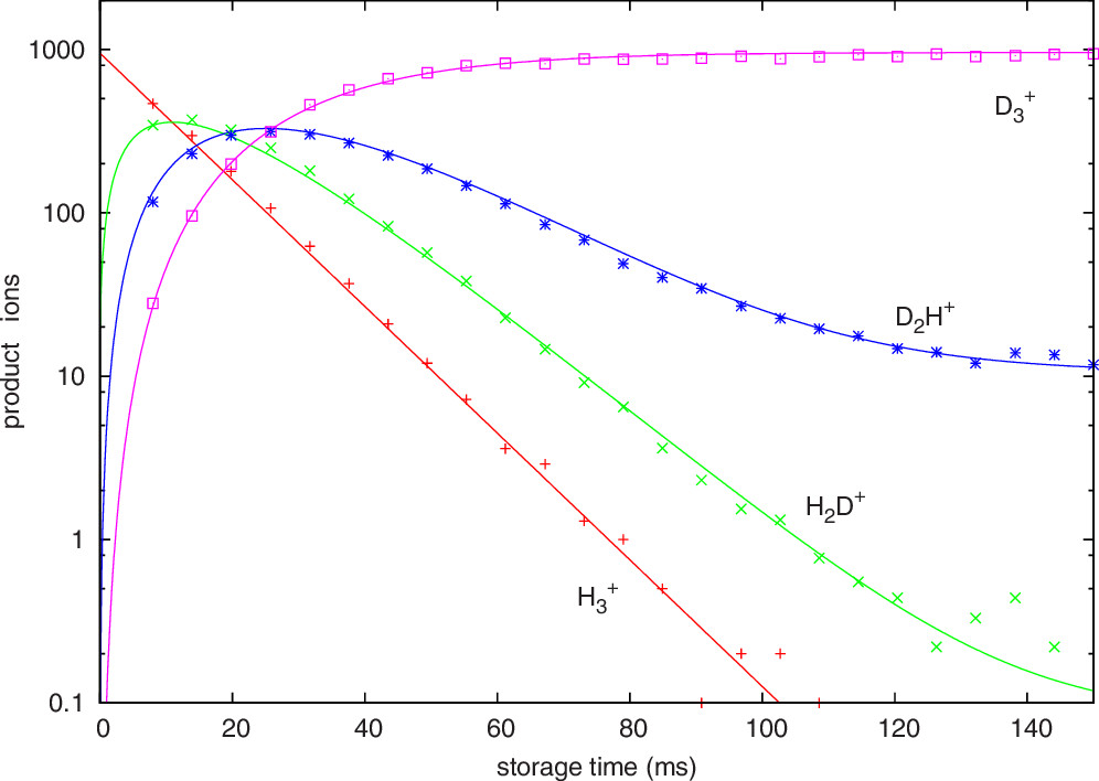
Our goal this week is to perform similar kinetic modeling to match this figure.
Kinetics
The deuteration of H\(_3^+\) proceeds through elementary reactions which occur in a single step. As a result, we can write down simple rate laws for each one of the reactions. In the table below, quantities in square brackets refer to the number density of a given species (molecules per cubic centimeter: units = cm\(^{-3}\)), and the second-order rate coefficients have units of cm\(^3\) s\(^{-1}\).
| Reaction | Rate (cm\(^{-3}\) s\(^{-1}\)) |
|---|---|
| H\(_3^+\) + HD \(\to\) H\(_2\)D\(^+\) + H\(_2\) | \(k_1^{(2)}\)[H\(_3^+\)][HD] |
| H\(_2\)D\(^+\) + HD \(\to\) D\(_2\)H\(^+\) + H\(_2\) | \(k_2^{(2)}\)[H\(_2\)D\(^+\)][HD] |
| D\(_2\)H\(^+\) + HD \(\to\) D\(_3^+\) + H\(_2\) | \(k_3^{(2)}\)[D\(_2\)H\(^+\)][HD] |
Under the experimental conditions, HD is present in large excess, so to a good approximation its number density remains constant. We can therefore rewrite these rates as pseudo-first-order reactions whose rates depend only on the number density of the ions. We can do this by defining new rate coefficients:
\[ k_n = k_n^{(2)}[\text{HD}] \]
With these new definitions, we can write the following rate equations for the concentrations of the ions:
\[ \frac{\text{d}[\text{H}_3^+]}{\text{d}t} = -k_1[\text{H}_3^+]\]
\[ \frac{\text{d}[\text{H}_2\text{D}^+]}{\text{d}t} = k_1[\text{H}_3^+] - k_2[\text{H}_2\text{D}^+]\]
\[ \frac{\text{d}[\text{D}_2\text{H}^+]}{\text{d}t} = k_2[\text{H}_2\text{D}^+] - k_3[\text{D}_2\text{H}^+]\]
\[ \frac{\text{d}[\text{D}_3^+]}{\text{d}t} = k_3[\text{D}_2\text{H}^+]\].
After some math (see the link below in further reading), we can derive these integrated rate equations for each molecule, where [H\(_3^+\)]\(_0\) is the starting number of H\(_3^+\) ions in the trap at \(t = 0\) (a value that the experimenters can choose).
\[ [\text{H}_3^+](t) = [\text{H}_3^+]_0e^{-k_1t} \]
\[ [\text{H}_2\text{D}^+](t) = \frac{[\text{H}_3^+]_0k_1}{k_2-k_1}\left(e^{-k_1t}-e^{-k_2t}\right) \]
\[ [\text{D}_2\text{H}^+](t) = \frac{[\text{H}_3^+]_0k_1k_2}{k_2-k_1}\left(\frac{e^{-k_1t}-e^{-k_3t}}{k_3-k_1} - \frac{e^{-k_2t}-e^{-k_3t}}{k_2-k_1} \right) \]
\[ [\text{D}_3^+](t) = [\text{H}_3^+]_0 - [\text{H}_3^+](t) - [\text{H}_2\text{D}^+](t) - [\text{D}_2\text{H}^+](t) \]
Our goal this week will be to determine the value of [H\(_3^+\)]\(_0\), as well as the second-order rate coefficients \(k_1^{(2)}\), \(k_2^{(2)}\), and \(k_3^{(2)}\) from the experimental data.