Week 3: Statistical Analysis of Experimental Data
Overview and Objectives
Python can be readily used to perform statistical analysis of experimental data. In chemistry, sophisticated statistical analysis is heavily used in applications involving health, nutrition, and medicine, but even in other areas of chemistry basic statistical analysis (computing standard errors, performing linear regressions, etc) is routine. This type of analysis often involves managing large amounts of data, handling missing data, and partitioning data into groups even before the analysis is run. Being able to comfortably organize and manipulate data is therefore very important.
This week we will explore three tools for managing and analyzing experimental data:
- pandas provides a set of classes for organizing, manipulating, and preprocessing data.
- scipy.stats provides low-level statistical functions and distributions.
- pingouin provides higher-level statistical analysis routines with an easy-to-use interface. We will be using these together with matplotlib to visualize and analyze data from the 2017-2018 CDC National Health and Nutrition Examination Survey (NHANES).
Background
Fundamentals of distributions
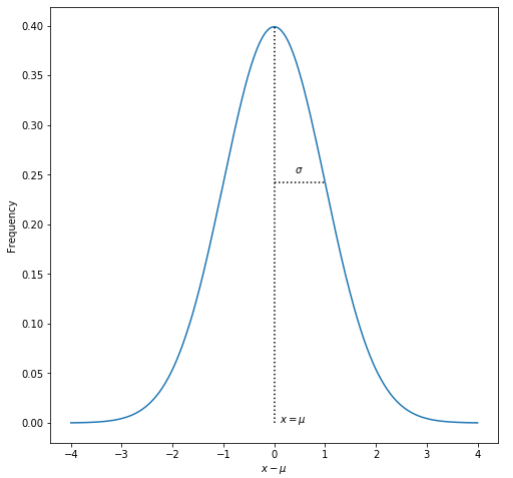
In week 1, we focused on using python tools to visualize “perfect” mathematical functions. Real experimental data, however, are subject to a variety of sources of noise: these could be for example from random errors in the measurements, the presence of undesired effects that compete with the desired effects, or heterogeneity in the subjects of the experiment. It is common to use descriptive statistics (mean, median, mode, standard deviation, etc) to summarize the distribution of experimental data. These are useful because the central limit theorem says that the distribution of many independent samples of nearly any random variable is given by the Normal Distribution. For instance, the heights of adult males in the US would likely follow a normal distribution very closely because each person’s height is determined by many, many competing factors. The normal distribution has the classic “bell-curve” shape with a mean of \(\mu\) and standard deviation \(\sigma\):
\[ f(x) = \frac{1}{\sigma\sqrt{2\pi}}\exp\left[{-\frac{1}{2}\left(\frac{x-\mu}{\sigma}\right)^2}\right] \]
However, most of the time, the “true” population mean and standard deviation are not known because it is impossible to observe every member of the population. In the NHANES data, for example, there are only about 9000 participants, while the US population is over 330 million. Instead, we can only make observations on a sample of the population. We can calculate the mean for the sample, and the exact value of this sample mean \(\bar{x}_s\) depends on which 9,000 people we included in the sample, and would change if we repeated the observations on a different sample. Te sample mean is
\[ \bar{x}_s = \frac{1}{N}\sum_i x_i \]
where \(N\) is the total number of samples and \(x_i\) is the value of sample \(i\). If we know the population mean \(\mu\), the true standard deviation (\(\sigma\), the square root of the variance \(\sigma^2\)) of our sample would be
\[ \sigma = \sqrt{\frac{1}{N}\sum_i(x_i-\mu)^2} \]
In most experiments, though, we can only estimate the mean from our sample \(\bar{x}_s\). If we want to estimate the population variance, we can apply Bessel’s correction to obtain the unbiased sample variance \(s^2\):
\[ s^2 = \frac{1}{N-1}\sum_i(x_i-\bar{x}_s)^2 \]
We can take the square root of the sample variance to obtain the sample standard deviation \(s\). The denominator in these equations is called the “degrees of freedom”. The number of degrees of freedom in a dataset is equal to the number of independent values in the set. A collection of \(N\) samples has \(N\) degrees of freedom, as long as all the samples are independent of one another. The set of squared differences from the population mean \((x_i-\mu)\) also has \(N\) degrees of freedom, because the population mean is independent of the samples. However, the set of squared differences from the sample mean \((x_i-\bar{x}_s)\) only has \(N-1\) degrees of freedom: given the sample mean and \(N-1\) of the \(x_i\) values, the remaining one can be calculated. We can say that one degree of freedom in the dataset was “used” to calculate the sample mean, and only \(N-1\) remain when we calculate the sample variance. Many of the scipy.stats functions that compute the variance take a ddof argument: when set to 1 (the default), the sample variance is estimated with \(N-1\) degrees of freedom, but this can be set to 0 if \(N\) degrees of freedom should be used.
Sometimes there is confusion about when to use \(N\) or \(N-1\) when calculating the variance. \(N\) should be used if the exact population mean is known or can be calculated. For instance, to compute the standard deviation of exam scores in a classroom, \(N\) would be used because the entire population consists only of students in the class who take the exam. Because the entire population was measured, the population mean \(\mu\) is measured directly. However, if you were to design a cognitive test and administer it to 1000 people, then use the results to estimate what the results would be for the population at large, \(N-1\) would be used when estimating the variance because the population mean is unknown.
The mean and variance are the first two moments of a distribution. The next two are skewness (which is related to the asymmetry of the distribution) and kurtosis (which is related to the heaviness of the tails of the distribution). The sample skewness and sample kurtosis can be calculated with scipy.stats, and if they significantly differ from the values for a normal distribution it may indicate that the data require further inspection. We will see an example in the second notebook.
Confidence Intervals and Statistical Hypothesis Testing
Because statistical distributions arise naturally in real systems, we can use properties of those distributions to determine how likely certain outcomes are by chance. The cumulative distribution function (CDF) shows what fraction of a distribution’s values fall between \([-\infty,x)\). So if the CDF for a given value of (x\) is 0.95, then 95% of the values of a distribution are less than \(x\), and there is only a 1 in 20 chance of observing a value of \(x\) or larger by chance. The CDF therefore allows us to construct confidence intervals. For instance, if 90% of values from a distribution fall in the range \([-x,x]\), then that range serves as a 90% confidence interval for the variable of interest.
Another use of the confidence interval is in performing a test of a hypothesis: for instance, determining whether the sample means of two sets of data points are meaningfully different. A statistical test ultimately results in the calculation of a p-value, which can be interpreted as the probability of obtaining a given result by random chance. Most statistical tests involve initially assuming that the null hypothesis is true: that there is no meaningful difference between the sample means, or to take an example from medicine, that a given treatment has no effect. The test involves computing a statistic, and comparing that statistic to a theoretical distribution to see how extreme the observed value is. The lower the p-value, the less likely it is to observe a result that is at least as extreme as the observed value. Together, p-values and confidence intervals provide descriptions of the data that, when used properly, can help guide its interpretation.
NHANES
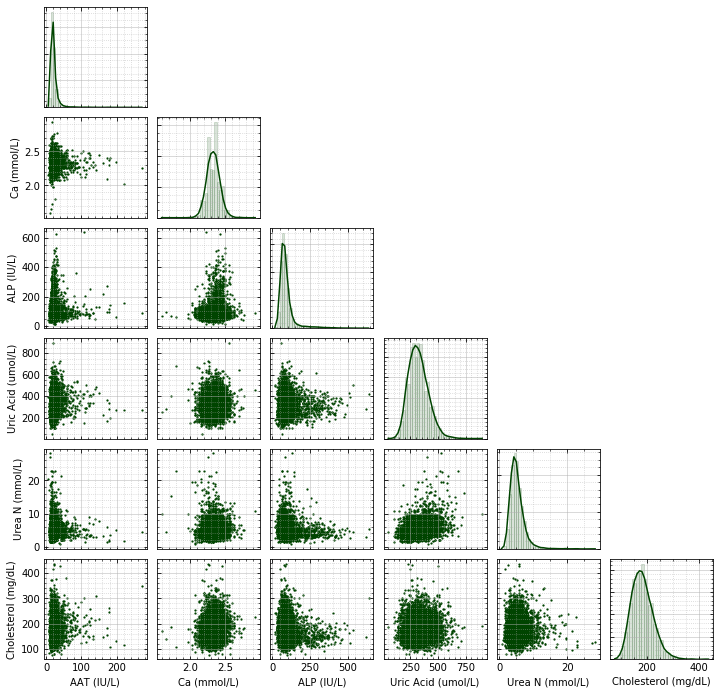
The NHANES survey consists of a combination of survey questions about a person’s health conditions, demographics, and dietary habits, as well as hard data from physical examinations and laboratory bloodwork tests. It has been performed since the 1960s, and is one of the main ways to track the national prevalence of diseases and other aspects of health and nutrition. The survey occurs on 2-year cycles, and contains data from several thousand people. It serves as the central data source for a large amount of the nutritional epidemiology in the US, and numerous scientific papers rely on it.
Further Reading
- Intro to pandas Data Structures
- 10 Minutes to
pandas - pingouin Guidelines
- Statistical Hypothesis Testing
- Linear Regression